How To Build A 3D Volume Renderer

Prof. Dr. Stefan Röttger, Stefan.Roettger@th-nuernberg.de

What is the scope of this lecture?

Volume data is a very common data type in medical visualization. It is generated by CT and MRI and PET computer tomography scanners, which are a powerful 3D sensing technique that has become an important standard in every day clinic routine.

In order to display that volume data, a so called volume renderer is required. In this lecture we are going to investigate the techniques and algorithms employed by a volume renderer. We also get in depth knowledge of the volume rendering principles by building a basic volume renderer by our own.

Lecture 1

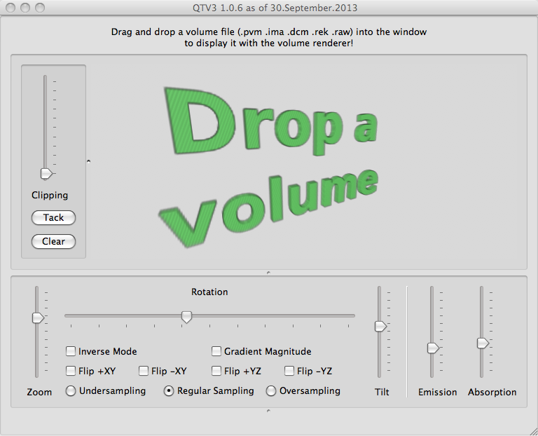
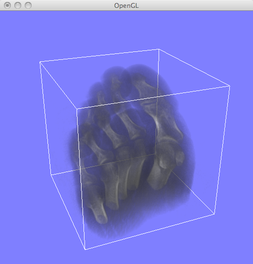
What is a volume renderer? We find out by trying one hands on.

• Installation of the QTV3
• Basic Usage of the QTV3
• Literature

Exercise: Get started with Unix and QTV3

Learning Objectives:

Objectives Test:

Lecture 2

Volume Rendering Prerequisites: Qt

• Qt Introduction
  • Qt Widgets
  • Qt Signal and Slots
  • QPainter Example
  • Qt Main Window
  • Qt Framework

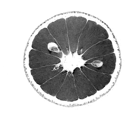
Exercise: Write a modularized Qt application that allows to open an image file via QFileDialog (e.g. this one: ). The file selector dialog should be triggered from the menu bar via signal/slot mechanism. Then the resulting image file is loaded into a QImage object via QImage::load() and displayed as the background of the main window with QPainter::drawImage() by overriding the widget’s paintEvent() method. Also show the image size in MB as text on top of the image.

Learning Objectives:

svn co svn://schorsch.efi.fh-nuernberg.de/qt-framework

Objectives Test:

Lecture 3

Volume Rendering Prerequisites: OpenGL

• QGL Introduction
• Graphic Concepts
• OpenGL Pipeline
  • OpenGL Terminology
  • OpenGL State
  • OpenGL Graphic Primitives
  • OpenGL Transparency
  • OpenGL ModelView Transformations
    • OpenGL Coordinate Systems
  • OpenGL Matrix Stack
  • Scene Graph To OpenGL
• Scene Graph APIs
• QGL Class Concept
  • QGL Example

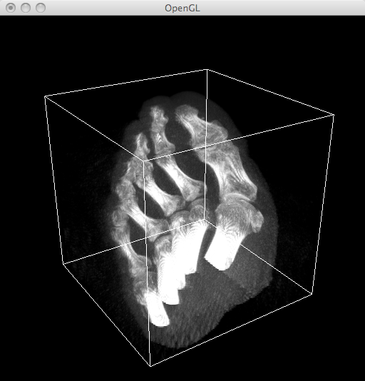
Exercise: Extend the Qt frame work with your own QGLWidget derived class that renders a stack of 10 semi-transparent and differently colored (yet untextured) slices within the unit cube (see this example rendering). Check the effect of enabling or disabling the Z-Buffer and blending. Let the camera rotate around the stack and make sure that the order of rendering is always from back to front. Raise the camera a bit so that you look down. Also use a wide angle and tele lens and tilt the camera. Lastly, put the rotating stack on a table with 4 legs using the matrix stack.

Learning Objectives:

Objectives Test:

Lecture 4

Volume Rendering Prerequisites: 3D Texturing

• OpenGL Texturing
  • Texture Space
  • Texture Coordinates
  • Texture Data
  • Texture Filtering
  • 2D Textures
• 3D Textures
  • Texture Coordinate Generation
  • 3D Texture Slice
  • 3D Texture Objects
  • 3D Texture Data
  • 3D Texture Example
  • 3D Texture Parameters
  • Marble Example
  • 3D Texture Interpolation Nearest Neigbour
  • 3D Texture Interpolation Trilinear

Exercise: Modulate the geometry of the previous exercise with a “checker board” 3D texture. Check both GL_NEAREST and GL_LINEAR texture filtering modes. Then render real Dicom data instead of the checker board texture (use the dicombase.h module of the frame work to load a Dicom series, e.g. the Artichoke series of the dicom-data repo). Implement a simple MPR (Multi-Planar Reconstruction) user interface that shows two axis-aligned slices through a dicom volume.

Learning Objectives:

Objectives Test:

Lecture 5

Direct Volume Rendering (DVR)

• DVR Principles
  • DVR Sampling
  • Optical Effects
• Ray Casting
• Slicing
  • Eye Centered Shells
  • View-Aligned Slices
  • View-Aligned Planes
• Axis-Aligned Cross Sections
  • Cross Section Example
  • Cutting Planes
• Tetrahedra
  • Tetrahedra Slicing
  • Tetrahedra Slicing Cases
  • Volume Slicing
  • 3D Vector Header
  • Slicing Case Table
  • Slicing Table as Switch
• Maximum Intensity Projection
  • MIP Example
  • MIP Syngo Example
• Bricking

Exercise: Render view-aligned slices instead of axis-aligned slices (use the slicer.h module of the frame work). Implement the MIP algorithm by using the according OpenGL blending mode.

Learning Objectives:

Objectives Test:

Lecture 6

Optical Model and Transfer Functions

• Optical Model
  • Absorption Coefficient
  • Absorption
• Numerical Integration
  • Integration with OpenGL
• Emission
  • Emission and Absorption
  • Windowing
• DVR Syngo Example
• Transfer Functions
  • TF Editor
  • Emission and Absorption with TF
• Isosurface Extraction
• DVR WebGL Example

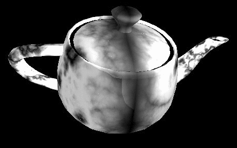
Exercise: Implement the MIP volume rendering technique by using view-aligned slicing. With that foundation, implement the DVR technique by using the according OpenGL blending mode (assuming a linear transfer function). Use the following helper modules:

• Dicom Framework
• Slicer Framework

With the artichoke dicom data the step by step implementation should look like the following:

Learning Objectives:

Objectives Test:

Lecture 7

Advanced Techniques:

• Pre- and Post- Classification
  • Ring Artifacts
  • Preintegration
  • Preintegration Example
  • Preintegration Quality
• Lighting
  • Gradient Calculation
• Gradient-Magnitude (GM)
  • Gradient-Magnitude Comparison
  • Gradient-Magnitude And MR
• Multi-Dimensional Transfer Functions
  • Spatialized Transfer Functions

Exercise: Show the difference of DVR and GM by using the QtV3 for a CT and a MR dataset.

Learning Objectives:

Objectives Test:

Course Certificate (PDF)